Chapter 7 · Matrices
Adjacency, Incidence and Laplacian
Three matrices for one graph, what each row/column product means, and the properties you can read off in O(1).
For a simple graph on V = {1, …, n}:
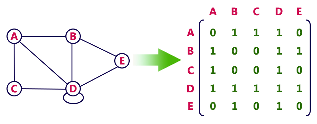
- adjacency A ∈ {0,1}n × n, Aij = 1 ⇔ ij ∈ E. Symmetric, zero diagonal, deg(i) = ∑j Aij.
- incidence B ∈ {0,1}n × m (undirected: Bie = 1 iff i is an endpoint of e) or {-1, 0, 1} for digraphs, with -1 at the tail.
- Laplacian L = D - A, where D = diag(deg). Equivalently L = B Bmathsf T for the oriented incidence matrix.
What each one is for
- A: walk counting, spectra, "is there an edge" queries (Counting Walks with Matrix Powers), and the semiring DP of Floyd–Warshall,
- B: cuts and flows — a column has exactly one -1 and one +1, so the flow conservation equations are B x = 0 and a cut is a row-space projection,
- L: everything involving spanning trees, random walks, and connectivity — xmathsf T L x = ∑uv ∈ E (xu - xv)2 ≥ 0, so L ≽ 0 always.
rank(L) = n - c, where c is the number of connected components, and ker L is spanned by the component indicator vectors.
xmathsf T L x = ∑uv ∈ E(xu - xv)2 = 0 ⇔ x is constant on every edge, hence constant on each component; so ker L has dimension exactly c. ∎
That one line is the reason the second-smallest eigenvalue of L (λ2, the algebraic connectivity / Fiedler value) measures how well connected G is: λ2 > 0 ⇔ connected, and Cheeger's inequality 2√(λ2) ≥ h ≥ λ2/2 ties it to the sparsest cut — which is the theoretical basis of spectral clustering and of "the Fiedler vector splits the graph well".
With B ∈ {0,1}n× m (no signs), BBmathsf T = A + D — not L. The signs are what make L = BBmathsf T work, and they are also what make the flow equations exact. For bipartite graphs the unsigned version equals 0 & M; Mmathsf T & 0-style structure that makes matching arguments transparent (Matching: Definitions and Duality).
#Reading properties off A in O(1)-ish
const int MAXN = 5000;
bitset<MAXN> adj[MAXN];
int common(int u, int v) { return (adj[u] & adj[v]).count(); }   // O(n/64)
ll triangles() {                                                  // O(n^3/64)
    ll t = 0;
    for (int u = 0; u < n; u++)
        for (int v : g[u]) if (v > u) t += (adj[u] & adj[v] & gt[v]).count();
    return t / 3;                                        // each triangle found at all 3 vertices
}tr(A3) = 6 · (#triangles) in a simple graph, and more generally tr(Ak) = ∑i λik counts closed walks, which is how one proves two graphs with different spectra are non-isomorphic (Trees: Six Definitions of One Object).
#Quotient matrices, an underrated tool
If the partition V = V1 ⊔ … ⊔ Vk is equitable (every vertex of Vi has the same number bij of neighbours in Vj), then the k × k matrix B = (bij) has the property that the largest eigenvalue of B equals that of A, and eigenvectors of B lift to A-eigenvectors constant on the parts. This is how one computes spectra of distance-regular graphs, Johnson graphs and the hypercube Qn (whose quotient is the path with self-loops on 0..n) in three lines instead of 2n.